.. note:: To download the tutorial data, use the following commands:

All tutorial data:

from recon.data import fetch_all_tutorial_data
fetch_all_tutorial_data(data_dir='./data')

Specific file (e.g., RNA data):

from recon.data import fetch_tutorial_data
fetch_tutorial_data('perturbation_tuto/rna.h5ad', data_dir='./data')

Predicting Treatment Effects with ReCoN

This tutorial demonstrates how to use ReCoN to predict the cell-type-specific effects of a molecular treatment. You will learn how to:

1. Build a multilayer network integrating GRNs and cell-cell communication

2. Select a molecule (ligand) to perturb

3. Predict direct effects (on receptor-expressing cells) and indirect effects (via cell-cell signaling)

4. Compare predicted responses across cell types

Use case: Given a therapeutic molecule (e.g., a ligand or antibody), predict which genes will be affected in each cell type and identify cell-type-specific responses.

import numpy as np
import scanpy as sc  # single cell data
import pandas as pd  # data manipulation
import liana as li  # cell communication
import recon  # multilayer and perturbation prediction
import recon.data

OMP: Info #276: omp_set_nested routine deprecated, please use omp_set_max_active_levels instead.

---

Setup

ReCoN uses single-cell RNA-seq data to infer cell-cell communication and gene regulatory networks.

Tip

The example data for this tutorial can be downloaded from the ReCoN repository.

Note

Required packages

This tutorial requires liana for cell-cell communication inference:

• Install with: pip install liana

rna = sc.read_h5ad("./data/perturbation_tuto/rna.h5ad")

Let’s check what cell types are present in this dataset

rna.obs["celltype"].unique().tolist()[:5]

['B_cell', 'ILC', 'Macrophage', 'MigDC', 'Monocyte']

---

Build the Multilayer Network

ReCoN integrates three main components:

1. Gene Regulatory Networks (GRNs) - TF → target gene relationships

2. Cell-Cell Communication (CCC) - Ligand-receptor interactions between cell types

3. Receptor-Gene Links - How receptors connect to intracellular signaling

1. Import Gene Regulatory Network

You can either generate GRNs directly with ReCoN or import a previously generated one.

Tip

If you wish to generate GRNs directly with ReCoN, please follow Tutorial 4: GRN Inference with HuMMuS.

Warning

GRN inference requires a Python 3.10 conda environment due to CellOracle dependencies. See the Installation guide for details.

grn_path = "./data/perturbation_tuto/grn.csv"
grn = pd.read_csv(grn_path)
grn = grn.sort_values(by="weight", ascending=False)[:500_000]
grn["source"] = grn["source"].str.capitalize()
grn["source"] = grn["source"] + '_TF'
grn["target"] = grn["target"].str.capitalize()
grn.head(3)

	Unnamed: 0	target	source	weight
0	0	Pax5	Mbd1_TF	0.000095
2	2	Pax5	Smad5_TF	0.000092
1	1	Pax5	Smad1_TF	0.000092

2. Compute Cell-Cell Communication

The cell-cell communication is inferred through LIANA+, an external package dedicated to this task.

Tip

For more information, check the LIANA+ documentation.

li.method.cellphonedb(rna, 
            # NOTE by default the resource uses HUMAN gene symbols
            resource_name="mouseconsensus",
            expr_prop=0.00,
            use_raw=False,
            groupby="celltype",
            verbose=True, key_added='cpdb_res')

Using resource `mouseconsensus`.
Using `.X`!
/pasteur/appa/homes/rtrimbou/miniconda3/envs/snakemake/envs/recon-grn/lib/python3.10/site-packages/anndata/_core/anndata.py:430: FutureWarning: The dtype argument is deprecated and will be removed in late 2024.
15364 features of mat are empty, they will be removed.
Make sure that normalized counts are passed!
/pasteur/appa/homes/rtrimbou/miniconda3/envs/snakemake/envs/recon-grn/lib/python3.10/site-packages/liana/method/_pipe_utils/_pre.py:146: ImplicitModificationWarning: Trying to modify attribute `.obs` of view, initializing view as actual.
/pasteur/appa/homes/rtrimbou/miniconda3/envs/snakemake/envs/recon-grn/lib/python3.10/site-packages/liana/method/_pipe_utils/_pre.py:149: FutureWarning: The default of observed=False is deprecated and will be changed to True in a future version of pandas. Pass observed=False to retain current behavior or observed=True to adopt the future default and silence this warning.
0.36 of entities in the resource are missing from the data.

Generating ligand-receptor stats for 1296 samples and 937 features

100%|██████████| 1000/1000 [00:04<00:00, 216.62it/s]

Format the LIANA output for ReCoN (rename columns to standard format):

Note

Required column names for ReCoN:

• source: ligand name

• target: receptor name

• celltype_source: cell type producing the ligand

• celltype_target: cell type expressing the receptor

• weight: interaction score (e.g., lr_means)

ccc_network = rna.uns["cpdb_res"].copy()
ccc_network = ccc_network[["ligand", "receptor", "lr_means", "source", "target"]]
ccc_network = ccc_network.rename(columns={
    "lr_means": "weight",
    "source": "celltype_source",
    "target": "celltype_target",
    "ligand": "source",
    "receptor": "target"
})
ccc_network = ccc_network[ccc_network['weight'] != 0]

ccc_network.head(3)

	source	target	weight	celltype_source	celltype_target
406685	App	Cd74	102.485008	cDC2	cDC1
405645	Copa	Cd74	102.370003	cDC1	cDC1
410237	Copa	Cd74	102.366211	eTAC	cDC1

3. Load Receptor-Gene Links

These links connect membrane receptors to downstream target genes in the GRN, enabling signal propagation from extracellular to intracellular networks.

receptor_genes = recon.data.load_receptor_genes("mouse_receptor_gene_from_NichenetPKN")
# for human, use "human_receptor_gene_from_NichenetPKN"

genes = np.unique(grn['source'].tolist() + grn['target'].tolist())
receptor_genes = receptor_genes[receptor_genes['target'].isin(genes)]
receptor_genes.head()

	source	target	weight
2	A1bg	Abca1	0.005156
3	A1bg	Abcb1a	0.005877
4	A1bg	Abcb1b	0.005877
7	A1bg	Acsl1	0.005915
8	A1bg	Adk	0.005092

---

Select a Molecule to Perturb

For treatment effect prediction, we need to choose a molecule (ligand) to simulate as a treatment. There are several strategies:

Strategy 1: Choose a receptor with high variance across cell types, then find its ligands.

This helps identify molecules that may have cell-type-specific effects:

# variance
ccc_network.groupby("target")["weight"].var().sort_values(ascending=False).head(3)

target
Cd74     932.779297
Cd68     155.465271
Itgal    152.500290
Name: weight, dtype: float32

Now identify the natural ligands of this receptor. You can either:

• Use a designed molecule targeting this receptor

• Choose one of its natural ligands from the cell communication network

ligands = ccc_network[ccc_network["target"]=="Cd74"]['source'].unique().tolist()
ligands

['App', 'Copa']

---

Run Treatment Effect Prediction

The multicell_targets function builds the multilayer network and runs Random Walk with Restart to predict treatment effects.

Note

Direct vs Indirect Effects

• Direct effect: Impact on cells that directly express the receptor for your molecule

• Indirect effect: Impact propagated through cell-cell communication from directly affected cells to other cell types

%%time
direct_effect, indirect_effect = recon.explore.multicell_targets(
        seeds=["Copa"],
        celltypes=["B_cell", "pDC", "Macrophage", "NK_cell", "T_cell_CD4", "T_cell_CD8"],
        grn=grn,
        receptor_grn=receptor_genes,
        ccc=ccc_network,
        grn_graph_weighted=True,
        receptor_grn_graph_weighted=True,
        receptor_graph_weighted=False,
        cell_communication_graph_weighted=True,
        cell_communication_graph_directed=False,
        restart_proba=0.6,
        extend_seeds=True,
        njobs=15
    )

Processing celltype 1/6: B_cell
Processing celltype 2/6: pDC

/pasteur/helix/projects/ml4ig_hot/Users/rtrimbou/ReCoN/src/recon/explore/recon.py:122: UserWarning: 
                No receptor_graph provided,
                an empty receptor graph will be created.
                

Processing celltype 3/6: Macrophage
Processing celltype 4/6: NK_cell
Processing celltype 5/6: T_cell_CD4
Processing celltype 6/6: T_cell_CD8

/pasteur/helix/projects/ml4ig_hot/Users/rtrimbou/ReCoN/src/recon/explore/recon.py:387: UserWarning: The celltypes dictionary was converted toa list of Celltype objects.
The keys of the dictionary will be the celltype names.

Computing intracellular contributions and direct effect...
Computing intercellular contributions and indirect effect...

  0%|          | 0/6 [00:00<?, ?it/s][Parallel(n_jobs=6)]: Using backend LokyBackend with 6 concurrent workers.
100%|██████████| 6/6 [00:00<00:00, 31.15it/s]
[Parallel(n_jobs=6)]: Done   2 out of   6 | elapsed:  1.1min remaining:  2.3min
[Parallel(n_jobs=6)]: Done   3 out of   6 | elapsed:  1.1min remaining:  1.1min
[Parallel(n_jobs=6)]: Done   4 out of   6 | elapsed:  1.2min remaining:   35.0s
[Parallel(n_jobs=6)]: Done   6 out of   6 | elapsed:  1.3min finished

CPU times: user 1min 2s, sys: 5.93 s, total: 1min 8s
Wall time: 2min 11s

---

Analyze Treatment Effects

View Direct and Indirect Effects

Direct effects: Genes affected in cells expressing the target receptor

direct_effect.head()

celltype_target	B_cell	pDC	Macrophage	NK_cell	T_cell_CD4	T_cell_CD8
gene
Zzz3	5.568139e-09	9.124538e-09	6.006453e-09	1.443905e-09	1.465908e-09	1.560960e-09
Zzef1	7.910818e-09	1.276460e-08	8.532004e-09	2.241151e-09	2.276372e-09	2.427962e-09
Zyx	2.311808e-08	2.538018e-08	2.369134e-08	2.052888e-08	2.055242e-08	2.059275e-08
Zyg11b	1.309827e-09	2.150962e-09	1.419632e-09	3.216471e-10	3.280418e-10	3.516321e-10
Zxdc	1.692286e-09	2.749142e-09	1.834584e-09	4.614275e-10	4.729096e-10	5.125789e-10

indirect_effect.head()

celltype_target	B_cell						pDC				...	T_cell_CD4				T_cell_CD8
celltype_source	B_cell	pDC	Macrophage	NK_cell	T_cell_CD4	T_cell_CD8	B_cell	pDC	Macrophage	NK_cell	...	Macrophage	NK_cell	T_cell_CD4	T_cell_CD8	B_cell	pDC	Macrophage	NK_cell	T_cell_CD4	T_cell_CD8
gene
Zzz3	7.760396e-13	1.363160e-14	1.044374e-14	3.864495e-15	3.308231e-15	3.894846e-15	1.189547e-14	1.292471e-12	1.741090e-14	7.543820e-15	...	1.090120e-14	5.014306e-15	3.703540e-13	5.171489e-15	9.401747e-15	1.659415e-14	1.279711e-14	5.898745e-15	5.182911e-15	4.402922e-13
Zzef1	1.032097e-12	2.167997e-14	1.462936e-14	4.876303e-15	3.561045e-15	4.477299e-15	1.598278e-14	1.844777e-12	2.322816e-14	9.321181e-15	...	1.410505e-14	5.392201e-15	4.702954e-13	5.585412e-15	1.191117e-14	2.415251e-14	1.715160e-14	6.699112e-15	5.532836e-15	5.562709e-13
Zyx	1.618271e-12	2.585074e-14	2.084081e-14	1.099187e-14	8.041645e-15	1.364838e-14	4.492823e-14	3.131443e-12	7.201589e-14	3.947233e-14	...	2.039161e-14	1.069780e-14	6.427157e-13	1.092050e-14	1.666707e-14	2.710333e-14	2.115135e-14	1.055248e-14	8.195229e-15	1.014019e-12
Zyg11b	5.348643e-13	7.700479e-15	6.028346e-15	2.836186e-15	2.123397e-15	2.913058e-15	6.033199e-15	7.885257e-13	7.826252e-15	3.810466e-15	...	3.306024e-15	1.499960e-15	2.344538e-13	1.989635e-15	5.479759e-15	8.888517e-15	6.859509e-15	3.435869e-15	2.977849e-15	4.643857e-13
Zxdc	3.455731e-13	4.689825e-15	3.212930e-15	1.931706e-15	1.274738e-15	1.452460e-15	5.061063e-15	1.132353e-12	1.440172e-14	3.223035e-15	...	4.276130e-15	1.979657e-15	2.148038e-13	2.091834e-15	3.257674e-15	5.661517e-15	4.910019e-15	2.249046e-15	2.049784e-15	2.335122e-13

5 rows × 36 columns

Indirect effects: Genes affected through cell-cell communication cascades

total_effect = recon.explore.combine_effects(direct_effect, indirect_effect, alpha=0.8)
total_effect.head()

celltype_target	B_cell	pDC	Macrophage	NK_cell	T_cell_CD4	T_cell_CD8
gene
Zzz3	0.000036	0.000030	0.000032	0.000036	0.000037	0.000036
Zzef1	0.000048	0.000043	0.000044	0.000051	0.000049	0.000047
Zyx	0.000085	0.000078	0.000071	0.000125	0.000129	0.000138
Zyg11b	0.000022	0.000017	0.000017	0.000028	0.000020	0.000032
Zxdc	0.000015	0.000023	0.000022	0.000021	0.000020	0.000018

Combine Direct and Indirect Effects

The combine_effects function merges direct and indirect effects using a weighting parameter α:

$$\text{Total Effect} = \alpha \times \text{Direct} + (1 - \alpha) \times \text{Indirect}$$

Tip

The default α = 0.8 gives more weight to direct effects, which has been empirically validated. You can adjust this based on your biological question.

%matplotlib inline
total_effect.plot.scatter(x='B_cell', y='pDC')

<Axes: xlabel='B_cell', ylabel='pDC'>

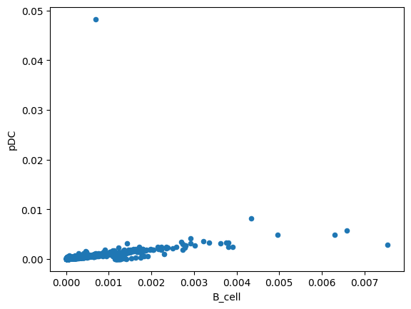
Visualize Cell Type Correlations

Scatter plots showing correlation of predicted effects between cell types:

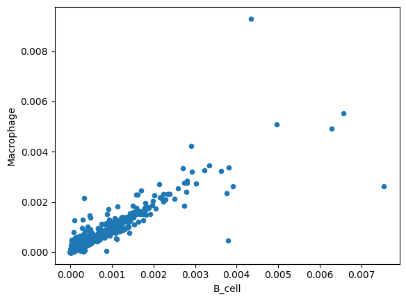
%matplotlib inline
total_effect.plot.scatter(x='B_cell', y='Macrophage')

<Axes: xlabel='B_cell', ylabel='Macrophage'>

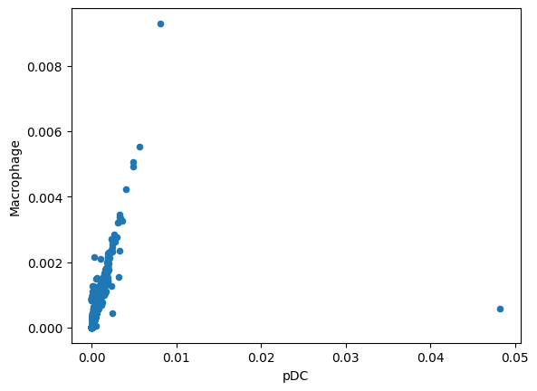
%matplotlib inline
total_effect.plot.scatter(x='pDC', y='Macrophage')

<Axes: xlabel='pDC', ylabel='Macrophage'>

---

Compare Cell-Type-Specific Responses

A key application of ReCoN is identifying differential responses between cell types. This helps understand:

• Which cell types are most affected by a treatment

• Which genes drive cell-type-specific responses

• Potential off-target effects on non-target cell populations

T cells CD4+ vs B cells

Compare predicted treatment response between T helper cells and B cells:

(total_effect["T_cell_CD4"] - total_effect["B_cell"]).sort_values(ascending=False)[:20]

gene
Fos       0.004969
Map4k1    0.004299
Ctnnb1    0.003570
Myc       0.003014
Ccnd1     0.002946
Arc       0.002888
Sucla2    0.002392
Cr2       0.002220
Ifng      0.002124
Rela      0.001742
Hmox1     0.001735
Il4       0.001699
Cdkn1a    0.001655
Chuk      0.001628
Nfkbia    0.001590
Bcl2l1    0.001563
Mapk9     0.001519
Il1b      0.001379
Egr1      0.001368
Vegfa     0.001333
dtype: float64

Note

Biological interpretation

Genes with higher scores in T cells CD4+ include known markers like Cd40lg, Cxcr4, and Cxcr6 - confirming that ReCoN captures biologically meaningful cell-type-specific signatures.

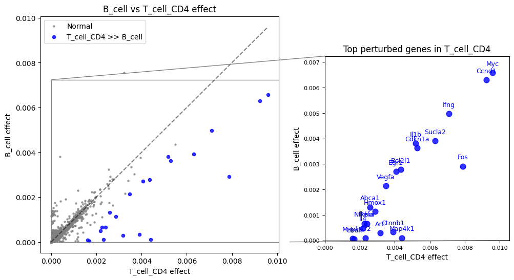
Visualize with a comparison plot highlighting the most differential genes:

recon.plot.plot_celltype_comparison(total_effect, "T_cell_CD4", "B_cell", quantile=0.998)

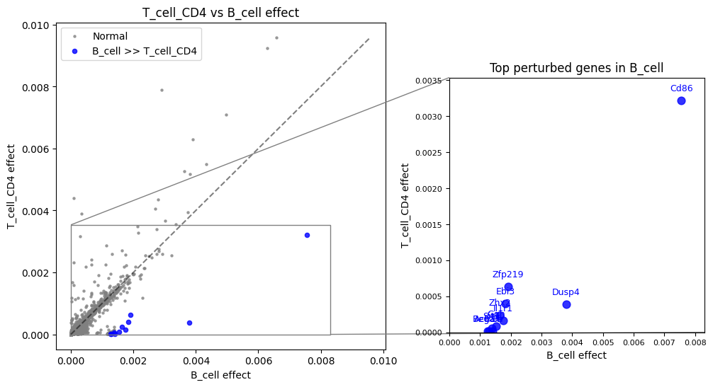
B cells vs T cells CD4+

Now look at genes with higher scores in B cells:

(total_effect["B_cell"] - total_effect["T_cell_CD4"]).sort_values(ascending=False)[:20]

gene
Cd86        0.004334
Dusp4       0.003410
Il1r1       0.001595
Ggh         0.001451
Ebi3        0.001430
Zhx2        0.001403
Il27        0.001391
Sit1        0.001321
Zfp219      0.001284
Actr1b      0.001268
Begain      0.001242
Smpd3       0.001242
Slc25a44    0.001241
Aptx        0.001230
Lipc        0.001223
Asb1        0.001221
Epcam       0.001220
Pmvk        0.001212
Mplkip      0.001203
Tdgf1       0.001192
dtype: float64

Note

Biological interpretation

Genes with higher expression in B cells include:

• Cd86: Marker of antigen presenting cells (including B cells)

• Ccr6: Classical marker of B cells, important for germinal center formation

References:

1. Suan D et al. (2017) Immunity 47(6):1142-1153. doi:10.1016/j.immuni.2017.11.022

2. Lee AYS & Körner H. (2019) Immunobiology 224(3):449-454. doi:10.1016/j.imbio.2019.01.005

recon.plot.plot_celltype_comparison(total_effect, "B_cell", "T_cell_CD4", quantile=0.999)

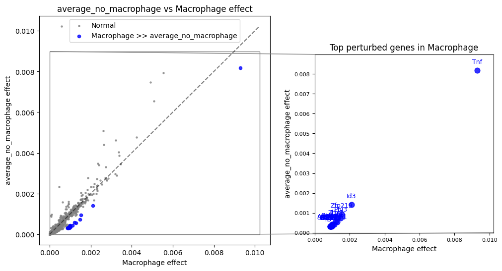
Macrophages vs Other Cell Types

Compare macrophage response to the average of all other cell types:

(total_effect["Macrophage"] - total_effect.loc[:, ~total_effect.columns.isin(["Macrophage"])].mean(1)).sort_values(ascending=False)[:20]

gene
Tnf         0.001129
Ebi3        0.000747
Il1r1       0.000734
Id3         0.000691
Ggh         0.000684
Timp2       0.000655
Il27        0.000654
Zhx2        0.000635
Sit1        0.000621
Arhgap31    0.000620
Actr1b      0.000598
Slc25a44    0.000597
Zfp219      0.000596
Begain      0.000584
Smpd3       0.000579
Aptx        0.000579
Lipc        0.000573
Pmvk        0.000567
Mplkip      0.000567
Asb1        0.000565
dtype: float64

Note

Biological interpretation

Macrophage-specific genes include markers of innate immunity and tissue remodeling:

• Tnf: Pro-inflammatory cytokine

• Tgfb1: Key regulator of tissue remodeling

• Mmp9: Matrix metalloproteinase involved in extracellular matrix degradation

total_effect["average_no_macrophage"] = total_effect.loc[:, ~total_effect.columns.isin(["Macrophage"])].mean(axis=1)
recon.plot.plot_celltype_comparison(total_effect, "Macrophage", "average_no_macrophage", quantile=0.998)
# delete to not include it by mistake later
del total_effect["average_no_macrophage"]

---

Gene Ranking Analysis

Compare Gene Ranks Across Cell Types

We can also compare the rank of each gene across different cell types to identify genes that are consistently high or show cell-type-specific rankings:

total_effect.rank().sort_values(by="NK_cell")[:10]

celltype_target	B_cell	pDC	Macrophage	NK_cell	T_cell_CD4	T_cell_CD8
gene
Ms4a4d	1.0	1.0	1.0	1.0	1.0	1.0
Hist1h2ac	2.0	2.0	2.0	2.0	2.0	2.0
Ifi27l2a	3.0	3.0	3.0	3.0	3.0	3.0
A3galt2	4.0	4.0	4.0	4.0	4.0	4.0
Hus1b	5.0	6.0	6.0	5.0	7.0	5.0
Kantr	6.0	5.0	5.0	6.0	5.0	6.0
Pcdhga6	9.0	7.0	7.0	7.0	6.0	8.0
Sugp1	7.0	9.0	8.0	8.0	10.0	7.0
Trim65	13.0	21.0	12.0	9.0	14.0	9.0
Tarm1	12.0	11.0	10.0	10.0	8.0	11.0

Tip

The top-ranked genes are often generic markers and metabolism-related genes that appear in all cell types. For biological interpretation, it’s usually more informative to focus on known markers or genes of interest specific to your system.

Focus on Known Cell Type Markers

Warning

Interpretation caveat

These predictions are for one specific ligand (Copa). The results don’t represent the actual expression state of your cells - they represent the predicted response to this specific perturbation. You won’t necessarily retrieve all cell-type markers.

Let’s check how known immune cell markers rank in each cell type:

markers = pd.Series([
    "Ptprc",   # pan-leukocyte (CD45)
    "Cd3e", "Trac",              # T cells
    "Cd4", "Cd8a",               # helper vs cytotoxic T
    "Ncr1", "Klrk1",             # NK cells
    "Ms4a1", "Cd19", "Cd79a",    # B cells
    "Sdc1",                      # plasmablasts/plasma cells
    "Lyz2", "Adgre1", "Csf1r",   # monocytes/macrophages
    "Itgax", "Zbtb46",           # conventional dendritic cells
    "Siglech",                   # plasmacytoid dendritic cells
    "Ly6g", "S100a8", "S100a9"   # neutrophils
])

markers = markers[markers.isin(total_effect.index).values]

total_effect.rank(ascending=False).loc[markers].sort_values(by="NK_cell")

celltype_target	B_cell	pDC	Macrophage	NK_cell	T_cell_CD4	T_cell_CD8
gene
Cd4	2391.0	274.0	273.0	53.0	2480.0	60.0
Cd19	492.0	814.0	797.0	398.0	365.0	407.0
S100a8	1304.0	1550.0	1499.0	641.0	787.0	639.0
Csf1r	1419.0	1781.0	586.0	669.0	725.0	655.0
S100a9	1503.0	1587.0	1557.0	696.0	710.0	710.0
Cd79a	876.0	1049.0	1142.0	750.0	757.0	734.0
Sdc1	1505.0	1414.0	1439.0	828.0	709.0	832.0
Itgax	1663.0	1948.0	1903.0	1168.0	1108.0	1095.0
Ptprc	1805.0	1935.0	1919.0	1826.0	1766.0	1606.0
Cd3e	3690.0	3482.0	3183.0	1988.0	1951.0	2100.0
Klrk1	547.0	503.0	549.0	2221.0	2104.0	2156.0
Lyz2	4595.0	3840.0	4159.0	5039.0	4668.0	5129.0
Zbtb46	5398.0	5408.0	5093.0	5368.0	5522.0	5602.0
Ms4a1	5631.0	6793.0	7326.0	5512.0	4492.0	5131.0
Cd8a	4227.0	6156.0	5033.0	5599.0	5480.0	4063.0
Ncr1	7048.0	7893.0	7954.0	6411.0	6168.0	6597.0

---

Summary

In this tutorial, you learned how to:

1. Build a multilayer network integrating GRNs, cell-cell communication, and receptor-gene links

2. Select a molecule to simulate as a treatment based on receptor variance

3. Predict treatment effects using multicell_targets() to get direct and indirect effects

4. Combine effects with the α parameter (default 0.8 for direct-weighted)

5. Compare cell-type responses to identify differential effects and cell-type-specific genes

Tip

Next steps

• Tutorial 2: Explore multicellular coordination around a pathway

• Tutorial 3: Visualize molecular cascades with Sankey diagrams

• Tutorial 4: Generate your own GRNs with HuMMuS